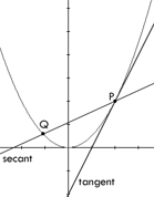
A tangent to a curve is a straight line
that touches the curve at a single point but does not intersect it at
that point. For example, in the figure to the right, the y-axis would
not be considered a tangent line because it intersects the curve at the
origin. A secant to a curve is a straight line that intersects
the curve at two or more points.
In the figure to the right, the tangent line
intersects the curve at a single point P but does not intersect the
curve at P. The secant line intersects the curve at points P and Q.
The concept of limits begins with the tangent
line problem. We want to find the equation of the tangent line to the
curve at the point P. To find this equation, we will need the slope of
the tangent line. But how can we find the slope when we only know one
point on the line? The answer is to look at the slope of the secant
line. It's slope can be determined quite easily since there are two
known points P and Q. As you slide the point Q along the curve, towards
the point P, the slope of the secant line will become closer to the
slope of the tangent line. Eventually, the point Q will be so close to
P, that the slopes of the tangent and secant lines will be
approximately equal.
A limit of a function is written as :

We want to find the limit of f(x) as x
approaches a. To do this, we try to make the values of f(x)
close to the limit L, by taking x values that are close
to, but not equal to, a. In short, f(x) approaches L
as x approaches a.
Examples
1
| Find the equation of the tangent line to the curve at point P
The previous example shows that the value a
can be approached from both the left and right sides. Each side has its
own limit. For example, as x approaches a from the
right side we have  and
as x approaches a from the left we have and
as x approaches a from the left we have  . .
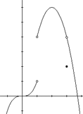
The graph to the right shows an example of a
function with different right and left hand limits at the point x = 1.
As x approaches 1 from the left side, the limit of f(x) approaches 1.
As x approaches 1 from the right side however, the limit of f(x)
approaches 4. In this case, the limit of f(x) as x approaches 1 does
not exist, because the left and right hand limits do not approach the
same value. This idea leads to the following theorem:

For the limit to exist, the left and right hand
limits must approach the same value. In our example, as x approaches 3,
the left and right hand limits both approach a value of 4. Since the
left and right hand limits are the same, the limit of f(x) as x
approaches 3 exists and is equal to 4. Even though the actual value of
f(3) is equal to 2, the limit is equal to 4. This gives the following
theorem:

Examples
2 |
Evaluate the limit, if it exists
Note: The example above
uses basic concepts that are covered in the sections below.
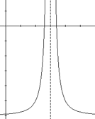
If a function is defined on either side of a,
but the limit as x approaches a is infinity or negative
infinity, then the function has an infinite limit. The graph of the
function will have a vertical
asymptote at a. A curve y=f(x) will have a vertical
asymptote at x = a if any of the following conditions hold:

Note: When dealing with
rational functions, often there is a vertical asymptote at values
of x that make the denominator equal to 0.
However, you must still show that one of the conditions above holds
true to prove that there is a vertical asymptote at that point. For example,
function f(x)=(x2-1)/(x-1) is undefined at x=1
but does not have a vertical asymptote at x=1. In fact, f(x)
= x+1 for all x≠1.
Examples
3
| Find the vertical asymptotes of the function
Calculating limits using graphs and tables takes
a lot of unnecessary time and work. Using the limit laws listed below,
limits can be calculated much more quickly and easily.
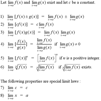
From the limit laws above, comes the property
of direct substitution. This property makes it possible to solve
most rational and polynomial functions. The property of direct
substitution states: For any rational or polynomial function f, if a is
in the domain of f then

Often, the method of direct substitution cannot
be used because a is not in the domain of f. In these
cases, it is sometimes possible to factor the function and eliminate
terms so that the function is defined at the point a. For an
example of factoring, see example 6 below.
Examples
4
| Evaluate the limit using limit laws
5
| Evaluate the limit using the property of direct substitution
6
| Evaluate the limit by factoring f(x) and eliminating terms
The squeeze theorem is an important concept that
will be very helpful in upper year calculus courses. The squeeze
theorem states:

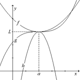
In simpler terms, the squeeze theorem states that
if the graph of g is squeezed between the graphs of f and h when x
is near a, and if f and h have the same limit L as x
approaches a, then the limit of g as x approaches a
is also L. The graph to the right illustrates the squeeze
theorem.
Note: The function g
does not have to be completely contained between f and h. It must only
be contained between f and h while x is near a. The
graph illustrates where the functions f and g cross each other.
Examples
7
| Evaluate the limit using the squeeze theorem
A function f is continuous at a number a
if:

Note: When proving that
a function is continuous, you may only show that the limit of f(x)
as x approaches a is equal to f(a). This
property implies that f(a) is defined and that the limit exists.
A function is continuous on an interval
if it is continuous at every number that falls within that interval.
Continuous functions have the following properties for simple
operations. If functions f and g are continuous at a, and c
is a constant, then the following functions will also be continuous at a:

A function is discontinuous at a
if it is defined near a but not continuous at a. To
prove that a function is discontinous, we must show which of the
requirements of continuous functions that it fails to hold for. There
are several different types of discontinuity, which are listed below.
Removable discontinuity: A function has
a removable discontinuity at a if the limit as x
approaches a exists, but either f(a) is different from
the limit or f(a) does not exist. It is called removable
discontuniuity because the discontinuity can be removed by redefining
the function so that it is continuous at a. In example #6
above, the function has a removable discontinuity at x = 3 because if
the function is redefined so that f(3) = -4/7, it will be continuous at
x = 3.
Infinite discontinuity: A function has an
infinite discontinuity at a if the limit as x
approaches a is infinite. In example #3 above, the function has
an infinite discontinuity at every point a = k*pi, since each point has
an infinite limit.
Jump discontinuity: A function has a jump
discontinuity at a if the left- and right-hand limits as x
approaches a exist, but are different. It is called jump
discontinuity because the function jumps from the left-hand limit to
the right-hand limit at each point. In example #2 above, the function
has a jump discontinuity at x = 0, since the right and left hand limits
approach different values.
Note: Polynomial
functions are continuous everywhere. Rational, root and trigonometric
functions are continuous at every number in their domain. In other
words, they are continuous wherever they are defined.
Examples
8
| Determine where the function is continuous
9
| Explain why the function is discontinuous at each point
The intermediate value theorem states: If f is a
continuous function on the closed interval [a, b] and N
is a number between f(a) and f(b), where f(a) does
not equal f(b), then there exists a number c in interval
(a, b) such that f(c) = N.
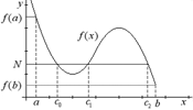
The intermediate value theorem simply says that
if a function is continuous on a closed interval [a, b],
and f(a) is different from f(b), then every value on the
y-axis between f(a) and f(b) has a corresponding value on
the x-axis between a and b.
Note: As the graph to
the right illustrates, there can be more than one value c in (a,
b) for a number N betwen f(a)
and f(b). The graph shows that there exist 3 numbers, c0,
c1 and c2, such
that f(c0)=f(c1)=f(c2)=N.
The intermediate value theorem is helpful when
proving that a root of a function exists in a certain interval.
Examples
10
| Show that the function has a root between a and b
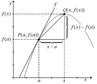
As explained at the beginning of this tutorial, a
tangent to a curve is a line that touches the curve at a single point,
P(a,f(a)). The tangent line T is the line through
the point P with the slope :

given that this limit exists. The graph to the
right illustrates how the slope of the tangent line is derived. The
slope of the secant line PQ is given by f(x)-f(a)/x-a.
As x approaches a, the slope of PQ becomes closer to
the slope of the tangent line T. If we take the limit of the
slope of the secant line as x approaches a, it will be
equal to the slope of the tangent line T.
The slope of the tangent line becomes much easier
to calculate if we consider the following conditions. If we let the
distance between x and a be h, so that x=a+h,
and substitute that equality for x in the slope formula, we get:

Note: Either of the
limit formulas above can be used to find the slope. You will obtain the
same answer using either formula.
These formulas have many practical applications.
They can be used to find the instantaneous rates of change of
variables. For example, if we use the formula above, the instantaneous
velocity at time t=a is equal to the limit of f(a+h)-f(a)/h
as h approaches 0.
Examples
11
| Find the equation of the tangent line to the curve at the point P
12
| Find the instantaneous rate of change
For more practice with the concepts covered in
the limits tutorial, visit the Limit Problems page at the link below.
The solutions to the problems will be posted after the limits chapter
is covered in your calculus course.
To test your knowledge of limits, try taking the general limits test on
the iLrn website or the advanced limits test at the link below.
Limit Problems
General Limit Test on iLrn
Advanced
Limit Test
|
Top of Page |
|

